Home Science Page Data Stream Momentum Directionals Root Beings The Experiment
The average of a set is a number, which in some way represents the middle of the set. Traditional Averages are the Mean, Median or Mode. There are many other types of averages. This notebook will discuss Decaying Averages in reference to Live Data Sets. Live Data Sets are Non-linear and Growing. {See Notebook on Live & Dead Data Sets.}
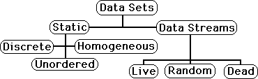
Traditional averages are preferable when dealing with Static Data Sets. A Static Data Set is a Data Set, which is Unordered, Discrete or Homogeneous. A Discrete Data Set is all-inclusive. It is complete – static, without growth. It might have happened all at once. In an Unordered Data Set the order of the data has no significance. A Homogeneous Data Set is one in which a sample set behaves like the whole set within certain limitations.
In a homogeneous set, a sample set behaves like the whole set. If we randomly select 2000 fourteen-year-old girls out of a total set of 2 million fourteen year old girls, the average height and weight for this sample set will be very similar to any other sample set of 2000 fourteen year olds from the same set. Therefore once the number of samples is above a certain limit, it doesn't matter if the researcher took 2000 or 200,000, the averages would be similar. (Of more critical importance is that his random sample is truly random.) Traditional Averages describe Homogeneous Sets adequately.
A Live Data Set is both growing and alive. It is a growing set of numbers that only ends with Death. Living Data Sets are normally associated with the movement through Time but don't necessarily need Time as a component. We will call Living Data Sets, Live Data Streams, because the Data never stops and so is never complete. Because it is not complete, it is not a Discrete Data Set.
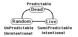
A Live Data Set, or Stream, is also alive. This means that the Data Stream is Unpredictable although exhibiting some Intentionality – Order. We will call a Live Stream Semi-Predictable. A Dead Data Stream is one in which the Data has become totally Predictable whether from Death or from a series of equations. A Random Data Stream is Unpredictable, but shows no Intentionality, Order. Some scientists don't believe in Living Data Streams because they believe that every phenomenon is ultimately reducible to an equation. Live Data Streams are not Homogeneous because they are alive and ever changing. Live Sets are not Static.
Below is a Diagram, which illustrates the relationship between the different types of sets. Static Sets, which traditional averages work best on, are also unordered. Data Streams are ordered, whether Live, Dead or Random.
This Diagram shows the differences between Live, Dead & Random Data Streams. They are all Data Streams and are not Static Data Sets, because each of these sets is ordered. Static Data Sets are unordered. A Dead Stream is not a Static Set because it is ordered. Note also that a Dead Stream transcends the polarity of Unintentional/Intentional, being neither or both. Much of science deals with Dead Streams. Successful Science is able to turn a Live Stream into a Dead Stream with a series of equations. Science attempts to Kill Live Streams. (I use these loaded words, i.e. Dead, Kill, Live, to describe these tightly defined mathematical concepts to poke fun, not to attack. I want to kill my attachments and my ego to die.)
The priorities are very different with Living Streams than with Static Sets. A representative sample means very little in a Live Stream. The most recent data samples are more important than distant data in describing the present state of affairs. To take a random selection of months from a person's life to describe how many hours he will sleep next month is relatively foolish from any perspective. The most recent months are the best predictor. The amount of hours an individual slept as a baby has very little to do with how much he sleeps as a full grown man, while the number of hours he has slept in the last few years would be a very good predictor. With a Live Data Set the most recent Data Bits have greater predictive ability while the most distant Data Bits have the weakest predictive ability. As soon as each Data Bit comes into existence in the Living Data Stream its impact begins to Decay. We want our Average to reflect this characteristic of our Live Data Sets. We want our average to reflect the decay of the data.
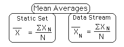
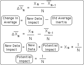
Because of the inherent unpredictability of Live Data Sets, we also want our averages to be sensitive to changes in recent Data Bits. Traditional Averages are insufficient to the task because they are cumulative. When applying the Traditional Mean to a Live Data Stream this is the equation we get. Note the lack of subscript for the Mean Average in the Static Set; it is fixed. The Mean Average of the Data Stream is not constant, however, because new data is always being added to the set. Our Living Data Stream is constantly increasing in size. Hence the Mean Average changes with each new entry.
The Change in the Mean Average is equal to the difference between the Impact of the New Data and the Inertia of the Old Average. This is a function of the size of the New Data bit, the Old Average, and the Number of elements in the sample. The Impact of the New Data equals the product of the New Data and the Potential Impact. The Potential Impact is defined as inversely proportional to N, the Number of elements in our Data Stream. N is always growing; hence the potential Impact is always shrinking for each new Data Piece in a Mean Average. {The top equation was derived in the Data Stream Momentum Notebook}.
Applying these equations to the Data Stream we notice that the Potential Impact of each subsequent piece of Data decreases. Because the Traditional Mean weights each Data Bit equally, the Potential Impact of each subsequent piece of Data diminishes through time. The opposite is true of Live Data Sets, where each moment has the same Potential Impact as the moment before. More recent Data Bits have just as much Potential for Impact on their time as did earlier Data Bits. The Mean Average declines in sensitivity with each new piece of Data.
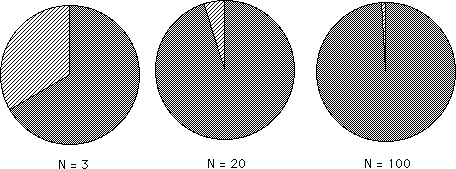
As N, the number of samples, continues to grow the potential impact of each new Data Bit falls. See diagram below. The area crossed by diagonal lines is the impact of the new data upon the old average. As is easily seen, the larger the N, the number of samples, the smaller the impact of the new data bit.
Because the potential Impact of each new Data Bit continues to shrink as time moves on, the sensitivity of Mean Averages continues to shrink.
Traditional Averages are insufficient in describing Live Data Sets. The study of Live Data Sets, which are growing, demands another approach. Traditional Averages are insufficient in describing Live Data Sets for two reasons. Traditional Averages deny Decay and lack Sensitivity to recent changes.